BigQuery Cost Optimization: A Practical Guide for Data and Engineering Teams
Kristóf Horváth, Rai Sudha Prabawa
30 min read
This is a comprehensive guide to BigQuery cost optimization, covering four tiers from quick configuration wins to reservation rightsizing to automated optimization. It includes SQL you can run against your own projects, and links to deeper dives on every topic along the way.
Your BigQuery bill grew again this month. You know the queries ran. You just don’t know which ones moved the bill, or what to do next. The cause is rarely one thing. A dashboard refreshes every few minutes against a large table with no date filter. A nightly pipeline re-reads two years of history to add one day. A reservation baseline sized for last quarter’s peak bills all night. None of these shows up as a standalone line item, and they all land on the same invoice. Teams that fix them one at a time also miss how the levers interact: a partition filter changes slot demand, which changes the right baseline.
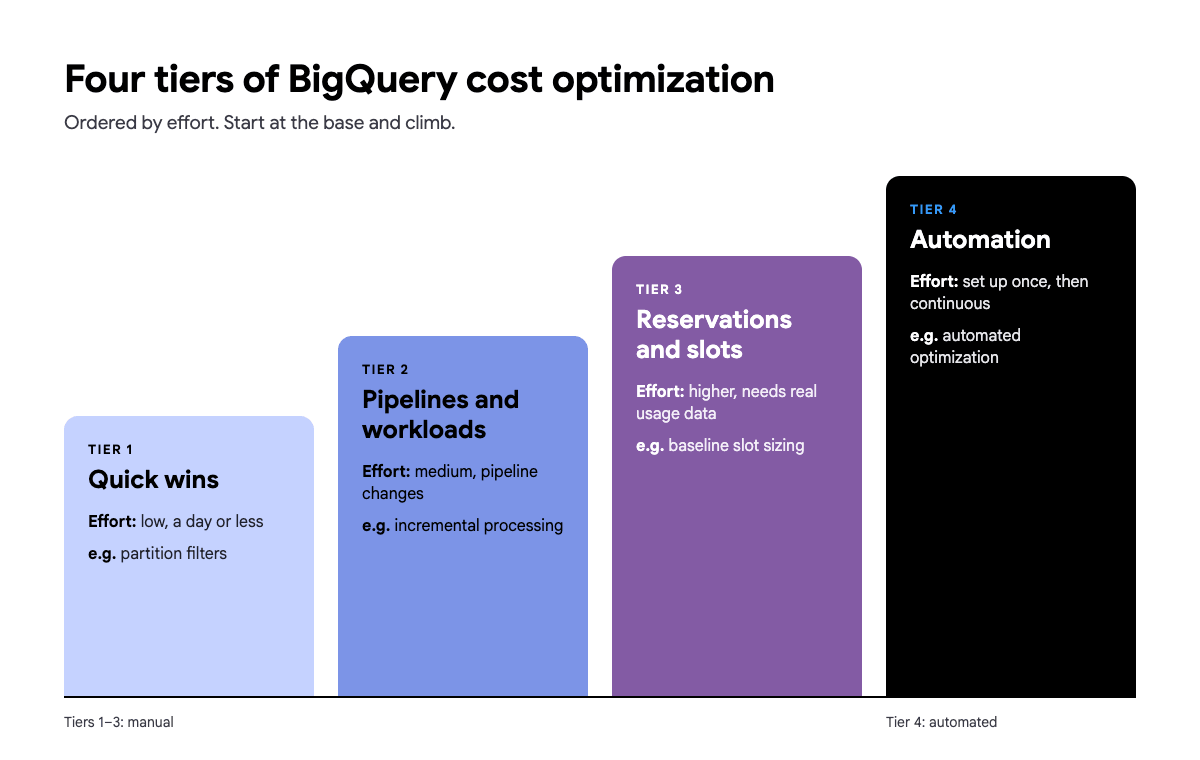
The guide is organized by effort, not by Google Cloud feature. Tiers 1 to 3 are manual: configuration and query fixes you can make in a day, pipeline and workload changes that take more thought, and reservation decisions that need real usage data. Tier 4 is where automation starts to matter. Wherever a number comes from a public dataset, you can paste the query and reproduce it yourself.
What causes unexpected BigQuery cost spikes?
Unexpected BigQuery cost spikes usually come from four main causes: queries that scan far more bytes than they return (on-demand), reservations sized or configured for capacity you don’t use (capacity pricing), pipelines that reload full tables instead of new data, and storage billed on the wrong model. Which one applies depends on your pricing model.
On on-demand pricing, the primary cost driver is bytes scanned: each query is charged for the data it reads. On capacity pricing, you pay for slots whether or not they are used, so the relevant signals are slot utilization, idle capacity, and autoscaling behavior. The four patterns below cover both. If you’re still deciding between the two models, Comparing BigQuery Pricing Models walks through the questions to ask.
Learn all about BigQuery Editions and Reservations. Download our white paper:

Bytes scanned, not rows returned (on-demand pricing)
Telltale sign: the bill jumps with no new workload shipped. Usually it is a new dashboard or scheduled query reading a big table without a date filter, or one that refreshes every few minutes. The query returns a handful of rows but reads the whole table.
BigQuery on-demand pricing charges for bytes read at query execution. A single unfiltered scan of a 10 TB table costs the same whether it returns 1 row or 1 million. The cost happens at scan time, which is why the fixes in Tier 1 focus on reading less. How Much Does a BigQuery Query Actually Cost? works through the arithmetic from 1 GB to 10 TB.
Slot waste and reservation misconfiguration (capacity pricing)
Telltale sign: the slot bill is the same at 3am as at noon, which points to a baseline sized for the peak rather than for typical demand. Or the bill spikes to the reservation’s ceiling whenever one heavy job runs.
On capacity pricing, slots you pay for but don’t use are silent waste. A baseline sized for the peak sits idle the rest of the day and still bills. A second, less obvious cause is a reservation set to “ignore idle slots”: it can’t borrow free idle capacity from its neighbours, so it autoscales and pays for demand it could have covered for free. Tier 3 covers the mechanics, and our post about BigQuery Slot Waste goes deeper on the overprovisioning patterns.
Full reloads and incremental gaps
Telltale sign: one pipeline gets a bit more expensive every month with no code change, because each run re-reads all the history it already processed.
Pipelines that reload entire tables instead of processing only new or changed data multiply bytes scanned unnecessarily, and the multiplier grows with every day of history. Tier 2 shows the measured difference.
Storage model mismatch
Telltale sign: the storage line grows faster than the data, or a dataset that is mostly compressible text or logs is still on the default logical billing.
Teams on logical billing storing compressible data can pay 2 to 3 times more than teams on physical billing. The default isn’t always the right choice, and it is one of the few cost levers that needs no query changes at all.
Two broader reads sit behind these four patterns: What Actually Drives BigQuery Costs? for the conceptual map, and The Hidden Costs of BigQuery for charges that fall outside them, such as streaming inserts, BI Engine, and BigQuery ML.
Learn more:
BigQuery Billing Explained: What Each Invoice Line Charges For
How do you reduce BigQuery costs? A four-tier BigQuery cost optimization framework
You reduce BigQuery costs by working through four tiers in order of effort: quick configuration and query fixes, pipeline and workload changes, reservation and slot tuning, and finally automation. Tier 1 changes take a day or less, Tiers 2 and 3 need workload data, and Tier 4 replaces manual review once it stops scaling.
- Tier 1, quick wins: storage billing model, partition filters, column selection, and clustering.
- Tier 2, pipeline and workload optimization: incremental processing, materialized views, and understanding what the query cache does and doesn’t cover.
- Tier 3, reservation and slot optimization: autoscale max, baseline slots and commitments, and idle slot sharing.
- Tier 4, automation: when manual review hits a ceiling, and what continuous optimization looks like.
What is the fastest way to cut BigQuery spend? Tier 1: Quick wins
These are changes any engineer can make in a day or less, often without touching query logic.
Choose the right storage billing model
Logical versus physical billing is set per dataset, not per table. A change takes about 24 hours to apply, and you can only switch a dataset once every 14 days, so treat it as a decision, not an experiment. See Google’s documentation on dataset storage billing models before flipping the setting.
The trade-off is straightforward. Logical billing costs more for stable, compressible data. Physical billing costs more for data that changes frequently. Teams storing heavily compressed or low-churn data often save significantly by switching to physical billing.
The reason high-churn tables cost more on physical billing is time travel and fail-safe storage. Under physical billing, every byte retained for the time travel window (7 days by default, configurable from 2 to 7 days) and the fail-safe window (an additional 7 days, not configurable) is billed as physical storage. Under logical billing, that historical and deleted data is not billed separately. So a table with heavy update and delete churn can look well compressed in its current state and still cost more on physical billing once time travel and fail-safe bytes are counted.
Here is a worked example. Take a table rebuilt from scratch every night: 3 TiB physical, about 10 TiB logical at typical compression. The numbers below use the active storage rates of $0.02 per GiB per month for logical and $0.04 per GiB per month for physical in the US multi-region (see BigQuery storage pricing to check rates for your region).
| Scenario | Billed storage | Approx. monthly cost |
|---|---|---|
| Logical billing | about 10 TiB logical | $205 |
| Physical billing, default 7-day time travel | about 45 TiB (current copy plus up to 14 retained old copies) | $1,843 |
| Physical billing, 2-day time travel | about 30 TiB (fail-safe stays at 7 days) | $1,229 |
As a rule of thumb for this table, physical billing stops paying off once more than about 5% of the data is rewritten per day: at 2% per day it comes to about $157 per month, and at 5% per day about $209, just above the $205 logical cost. These figures price everything at the active rates and assume the full retention window is kept, so treat them as an upper estimate, not a universal number. Rates and compression ratios vary by table and region.
Learn more:
BigQuery Logical vs Physical Storage Pricing: How to Choose
Partition pruning: the cost of a missing WHERE clause
Partition filters prevent BigQuery from scanning partitions that are irrelevant to the query. A query on a date-partitioned table without a date filter scans every partition. If your table isn’t partitioned yet, that is also an argument for partitioning it.
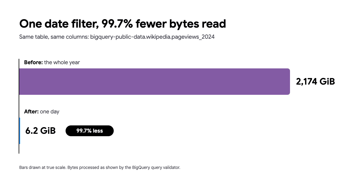
You can check the numbers below yourself. They were measured on Google’s public Wikipedia pageviews table (bigquery-public-data.wikipedia.pageviews_2024), and the query validator in the BigQuery console shows bytes processed before you run anything.
-- Before: the whole yearSELECT title, viewsFROM `bigquery-public-data.wikipedia.pageviews_2024`WHERE datehour >= '2024-01-01';-- 2,174 GiB
-- After: one daySELECT title, viewsFROM `bigquery-public-data.wikipedia.pageviews_2024`WHERE datehour >= '2024-01-15'AND datehour < '2024-01-16';-- 6.2 GiB, 99.7% less (one month is 188 GiB)
At the on-demand rate of $6.25 per TiB in the US multi-region (check pricing for your region), that is roughly $13 per run against about 4 cents.
There is a guardrail worth copying. This table has require_partition_filter switched on, so it won’t run at all without a date filter. It is the cheapest protection you can add to your own large tables: it turns a missing filter into a query error instead of a silent full scan.
One gotcha: pruning stops working when the filter value comes from a subquery. Google’s documentation says to filter the partitioning column with a constant expression, because a dynamic value such as a subquery prevents pruning. On this table, you see it straight away: a subquery filter is rejected, because require_partition_filter finds no filter it can use for partition elimination. On a table without that guardrail, the same query runs and scans every partition. A function applied directly to the partition column, like DATE(datehour) = '2024-01-15', still prunes (see the supported functions list), so it is specifically the subquery case that breaks it. A dry run tells you before you pay.
Learn more:
BigQuery Partitioning: How It Works, Cost and SQL Examples
Remove SELECT *: columnar pricing basics
BigQuery charges for every column a query reads, including columns used only in filters and joins, not just the ones in the SELECT list. SELECT * on a wide table reads every column even if the application only needs two.
A common misconception is that LIMIT reduces cost. On a normal (non-clustered) table, BigQuery still scans every byte of every column the query touches before applying the limit. LIMIT only reduces the rows returned to the client, not the bytes billed.
Related, and smaller: every table referenced in a query is billed a minimum of 10 MB, even if the query reads less (on-demand pricing details). A tiny lookup table in a join isn’t a major cost driver on its own, but it adds up across queries that join many small tables.
Google’s public Stack Overflow questions table (bigquery-public-data.stackoverflow.posts_questions, 20 columns, 37 GiB) shows that which columns you read matters more than how many:
SELECT * FROM `bigquery-public-data.stackoverflow.posts_questions`;-- 37.2 GiB
SELECT * FROM `bigquery-public-data.stackoverflow.posts_questions` LIMIT 10;-- 37.2 GiB, LIMIT changes the rows returned, not the bytes read
SELECT id, title, score FROM `bigquery-public-data.stackoverflow.posts_questions`;-- 1.6 GiB
SELECT * EXCEPT (body) FROM `bigquery-public-data.stackoverflow.posts_questions`;-- 3.7 GiB, one text column is 90% of the table
The last query is the interesting one: dropping a single long text column removes 90% of the bytes. The second query is also the real-data proof for the LIMIT misconception, since LIMIT 10 reads the exact same 37.2 GiB as no limit at all.
Don’t generalize this to “reading N of 100 columns costs proportionally less.” That only holds if the columns are similar in size. Here, 3 of 20 columns read just 4% of the bytes because the excluded columns include one dominant text column. The lesson is to know which columns are big, not that fewer columns is always proportionally cheaper.
If you only want to look at rows, the table preview in the BigQuery console is free and doesn’t run a query.
This is the Tier 1 win that takes the most effort to enforce, because it requires reviewing existing queries rather than changing a setting. A linting step in CI or a periodic query review pass is the practical way to keep it from creeping back.
Clustering basics
Clustering sorts table data by one or more columns, which lets BigQuery skip blocks that don’t match your filter predicates. Unlike partitioning, clustering works well on columns with many distinct values (user IDs, event types, project IDs), and you can combine up to four columns.
The Wikipedia pageviews table from the partitioning example is clustered by (wiki, title), so one table shows both the single-column effect and why column order matters. All three queries below read the same one-day partition, and the numbers are measured billed bytes.
-- No filter on a cluster column: 6.22 GiBSELECT SUM(views)FROM `bigquery-public-data.wikipedia.pageviews_2024`WHERE datehour >= '2024-01-15' AND datehour < '2024-01-16'AND LENGTH(title) > 0;
-- First cluster column: 1.03 GiB (83% less)SELECT SUM(views)FROM `bigquery-public-data.wikipedia.pageviews_2024`WHERE datehour >= '2024-01-15' AND datehour < '2024-01-16'AND wiki = 'en' AND LENGTH(title) > 0;
-- Both cluster columns: 0.10 GiB (98% less)SELECT SUM(views)FROM `bigquery-public-data.wikipedia.pageviews_2024`WHERE datehour >= '2024-01-15' AND datehour < '2024-01-16'AND wiki = 'en' AND title = 'Albert_Einstein';
The LENGTH(title) > 0 condition only exists so that all three queries read title and views for a fair comparison. The second and third also read wiki for the filter.
Column order matters. Filtering on title alone (the second cluster column, without wiki) reads 2.24 GiB: 64% less than no filter, but far less effective than filtering on the first cluster column (83% less). List the column your readers filter on most often first when you cluster a table.
Tier 2: Pipeline and workload optimization (moderate effort)
These optimizations take more effort: understanding workload patterns, pipeline architecture, and how BigQuery caches and materializes results.
Incremental processing vs. full reloads
Pipelines that truncate and reload a destination table on every run re-scan source data that hasn’t changed. Incremental patterns (for example MERGE, or INSERT INTO ... WHERE event_date > last_run) cut the bytes processed per run, and the gap widens as history grows.
Here is a measured example. Rebuilding a daily rollup of the first half of 2024 from the public Wikipedia pageviews table, the way a full-reload pipeline would have run on 30 June, reads 577.7 GiB per run, about $3.53 at the on-demand rate in the US multi-region (check pricing for your region). In a real pipeline that number grows every day, because the history it re-reads keeps growing (the full year of those three columns is 1,174 GiB). Adding only the new day reads 2.9 GiB, 99.5% less. A 3-day lookback window to catch late-arriving data reads 8.7 GiB, 98.5% less. @run_date is a query parameter your scheduler supplies.
-- Full reload, every runCREATE OR REPLACE TABLE reporting.daily_wiki_viewsPARTITION BY view_date ASSELECT DATE(datehour) AS view_date, wiki, SUM(views) AS viewsFROM `bigquery-public-data.wikipedia.pageviews_2024`WHERE datehour >= '2024-01-01' AND datehour < '2024-07-01'GROUP BY view_date, wiki;
-- Incremental, new day onlyINSERT INTO reporting.daily_wiki_views (view_date, wiki, views)SELECT DATE(datehour), wiki, SUM(views)FROM `bigquery-public-data.wikipedia.pageviews_2024`WHERE datehour >= TIMESTAMP(@run_date)AND datehour < TIMESTAMP(DATE_ADD(@run_date, INTERVAL 1 DAY))GROUP BY 1, 2;
If you use a MERGE instead of a plain incremental INSERT, add a filter on the target table’s partition column to the ON clause, for example AND t.view_date >= DATE_SUB(@run_date, INTERVAL 2 DAY). Without it, the MERGE reads the entire target table to find matches, which can cancel out the saving the incremental source filter just achieved. An unfiltered WHEN NOT MATCHED BY SOURCE clause forces the same full scan on the target side.
The same trap shows up in dbt. Setting incremental_strategy = 'insert_overwrite' together with partition_by replaces whole partitions instead of matching rows, which avoids the target-table scan described above. dbt’s own documentation is direct about the default alternative: the merge strategy “requires scanning all source tables referenced in the model SQL, as well as destination tables.”
Learn more:
BigQuery Optimization: From Full Reload to Incremental Processing
Materialized views: when they save money and when they cost more
A materialized view (MV) pre-computes and stores the result of a query. BigQuery can then automatically use the MV to answer matching queries on the base table, so downstream queries get cheaper without being rewritten. That is the main reason MVs save money in practice: existing dashboards and pipelines that already query the base table get cheaper with no code change. Note that the MV itself has storage costs and refresh overhead.
The trade-off: MVs save money when the same expensive aggregation is queried repeatedly. They add cost when the base table updates frequently (refresh cost) or when the MV is rarely queried relative to its maintenance overhead.
To keep the numbers teachable, the worked example below assumes the daily queries explicitly target the MV, rather than modeling BigQuery’s automatic query rewrite. Rewrite is real and is why MVs work well in production, but it isn’t fully predictable or simple to price in a before/after comparison. The figures use the US multi-region on-demand rate of $6.25 per TiB (check pricing for your region).
Scenario A, base table only receives new events. A 5 TiB events table receives new events all day. A dashboard runs a daily aggregation 50 times a day, each run reading about 1 TiB of the columns it needs: 50 TiB a day, or $9,375 per month querying the base table directly. With an MV, refreshes read only the new events (about 10 GiB per day), the 50 queries read the 2 GiB MV, and storage is 2 GiB. That comes to about $20 per month.
Scenario B, base table is rewritten. If the base table is rewritten rather than appended to (a full reload or a MERGE every half hour, say), each refresh has to recompute everything. At the default refresh cadence of at most every 30 minutes, that is up to 48 full recomputes a day (about 1 TiB each), or roughly $9,000 per month. If the dashboard is only opened twice a day, querying the base table directly would have cost $375 per month, far cheaper than the MV.
| Scenario | Querying the base table directly | With an MV |
|---|---|---|
| A: appended all day, 50 dashboard queries a day | $9,375 per month | about $20 per month |
| B: rewritten, 48 refreshes a day, 2 dashboard queries a day | $375 per month | about $9,000 per month |
The general rule: an MV pays off when queries/day × bytes per base-table query is bigger than refresh bytes/day + (queries/day × bytes per MV query). That is the formula behind “save when queried repeatedly, cost more when refreshed frequently relative to how often it’s read.”
Two caveats:
- First, the “costs more” case is our model, not an official spec: Google doesn’t document exactly how updates and deletes affect refresh cost, so treat Scenario B as an estimate rather than a guaranteed number.
- Second, querying the base table directly only costs what it does in Scenario A because data arrives all day. On a table loaded once a day, BigQuery’s query cache would make 49 of the 50 daily queries free, which would change the comparison significantly. The next section covers why.
Query caching: what it does and what it doesn’t cover
You can rely on the query cache for dashboards over tables loaded once a day: after the first refresh, most repeat views are free. You can’t rely on it for tables that receive data all day, because every load invalidates it. So there is no need to build your own result cache for daily-batch tables (BigQuery already does it), and for constantly changing tables a materialized view, from the previous section, is the better tool.
The underlying facts: results are kept for about 24 hours on a best-effort basis (not guaranteed), and a cache hit isn’t charged as a query at all. The cache is per-user and per-project by default. Results are shared between different users of the same project only on Enterprise and Enterprise Plus editions, which matters for dashboards that run queries as a shared service account rather than as individual users.
The cache is skipped when:
- the query uses non-deterministic functions such as
CURRENT_TIMESTAMP()orRAND() - a referenced table has changed since the last run
- the parameters differ, even if the query is structurally identical
- the query text differs in any way, including whitespace or comments
- the job writes its results to a destination table
- a referenced table has recently received streaming inserts
- the query uses wildcard tables, external data sources (other than Cloud Storage), or tables protected by row-level security
Tier 3: Reservation and slot optimization
This tier is about configuration decisions at the reservation layer. It stays conceptual, with links to deeper posts for the details.
The three subsections below are not sequential steps. A common playbook reads “commit to a baseline, then add autoscaling, then share idle slots,” which only fits teams with predictable workloads. Many teams have spiky or unpredictable workloads, and for them the better starting point is a reservation with zero baseline and only an autoscale max. The commitment comes later, once they know their floor. So autoscaling-only comes first here, baseline is the refinement for teams that already see a stable floor, and idle slot sharing comes last because it only applies once you have baseline slots to lend.
Autoscaling and the autoscale max: the safe default when you don’t know your workload yet
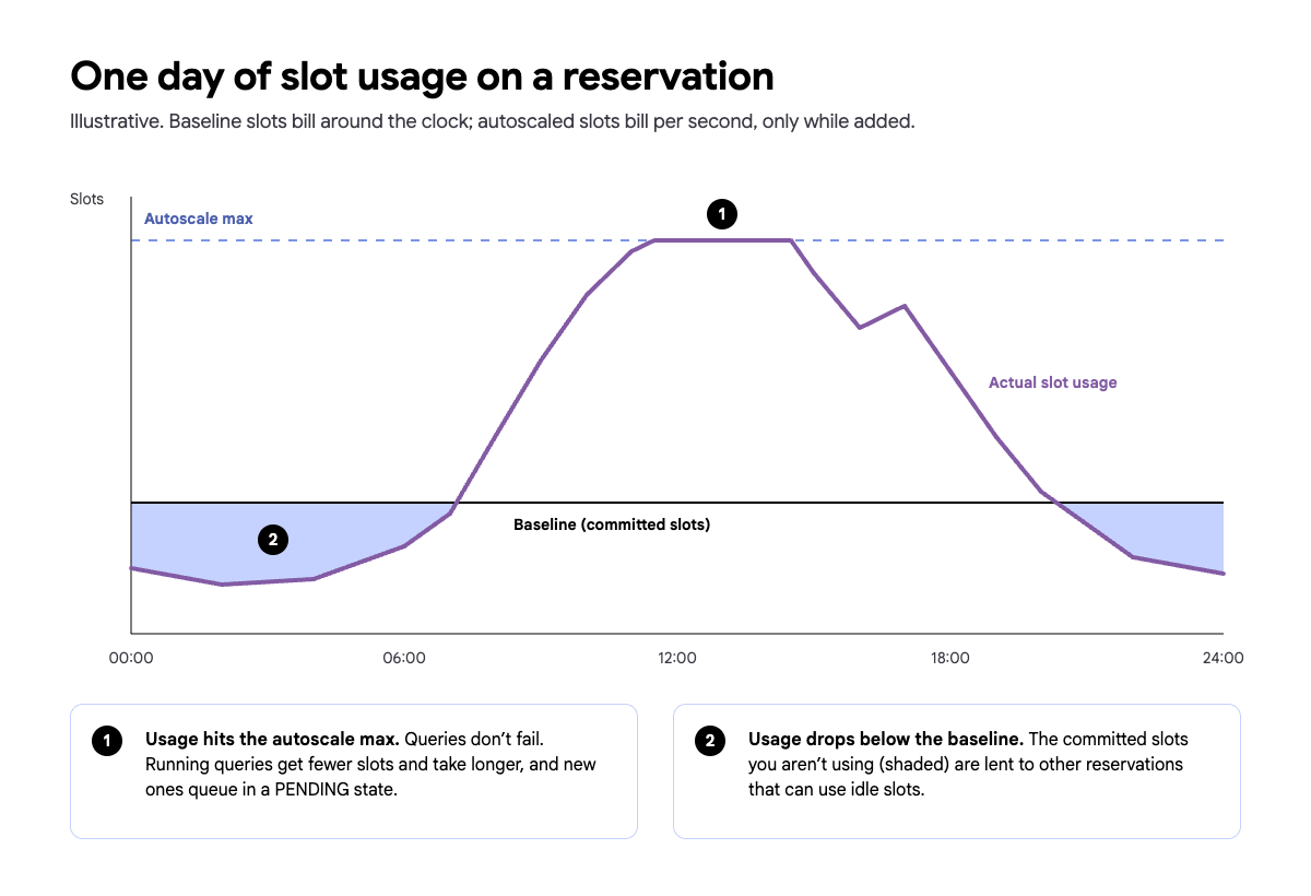
You can run a reservation with zero baseline and only an autoscale max. This is the safest starting point if you don’t know your workload yet: the reservation scales up to the ceiling you set when queries need capacity, and there is no idle baseline commitment sitting unused.
A reservation with a baseline of zero holds no capacity while no queries are running, so overnight there is no idle baseline to pay for. When queries arrive, it adds slots up to the autoscale max. Scale-up is rounded up to the nearest 50 slots, and you are charged for the slots it scaled to, not for the slots your queries actually used, so the bill follows demand rather than a fixed commitment. That is the mechanical reason this is the safe starting point. Google documents the model in its introduction to slot autoscaling.
The trade-off: autoscaled slots aren’t reserved in advance, so their availability depends on current capacity in the region. That is why Google recommends a non-zero baseline when you need the most predictable performance. Zero baseline trades some of that predictability for no idle cost. Also note that the maximum size of a reservation is bounded by the regional slot quota, which defaults to anywhere from 1,000 to 10,000 slots depending on the region. You can request an increase.
The autoscale max caps how far the reservation can expand. Set it too high and you are exposed to runaway slot consumption on an unexpectedly large job. Set it too low and workloads are starved at peak. If you also want to cap slots borrowed from other reservations, see the reservation scaling modes post.
By default, queries don’t fail at the ceiling. Running queries get fewer slots and take longer. Once the reservation reaches its concurrency limit, new queries wait in a PENDING state, and by default interactive queries that haven’t started within 6 hours time out.
Two signals tell you the ceiling is set too low:
- Queue time grows at peak hours. Compare
start_timewithcreation_timeinINFORMATION_SCHEMA.JOBS. - Slot usage sits flat at the max for long stretches. The hourly slot-utilization query in Monitoring slot utilization below is what surfaces this.
Learn more:
BigQuery Reservations: How Does Autoscaling Really Work?
Setting a baseline slot commitment: the next step once you see a stable floor
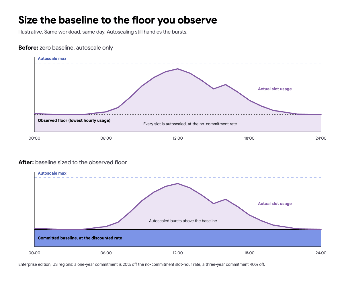
On-demand pricing charges per byte scanned. Capacity pricing charges per slot-hour. And a baseline on its own does not save money: it costs the same per slot-hour as autoscaling. The saving comes from committing it. Slot commitments exist only on Enterprise and Enterprise Plus editions; Standard edition has none.
Here is how the rates compare in the US multi-region (from Google’s BigQuery pricing page; check pricing for your region and edition). Standard edition, for reference, is $0.04 per slot-hour pay-as-you-go.
| Enterprise edition, US multi-region | Per slot-hour |
|---|---|
| Autoscaling or baseline, no commitment | $0.06 |
| One-year commitment (20% off) | about $0.048 |
| Three-year commitment (40% off) | about $0.036 |
Once a team has run on autoscaling long enough to have real usage data, four questions size the baseline decision. They are questions rather than a formula, because there is no universal threshold:
- Floor: what is the lowest hourly slot usage over the last 2 to 4 weeks, nights and weekends included? The hourly query in Monitoring slot utilization below surfaces it.
- Peaks: how much of the day do you spend above that floor? Short peaks are cheaper left to autoscaling than baked into a larger baseline.
- Commitment length: will the workload still look like this in one or three years? A commitment can’t be deleted while it is active, though it can be converted to a longer one.
- Neighbours: do other reservations in the same admin project need capacity when yours is quiet? Idle baseline slots get lent to them, which leads into the next section.
For a closer look at sizing, see how to find a right-sized commitment. If you already hold a commitment, running some queries on-demand can cut autoscaling costs, and the BigQuery Editions comparison covers which edition’s rates and features apply to you.
Learn more:
How to Configure BigQuery Baseline Slots and Slot Commitments
Idle slot sharing and reservation groups
Idle slots are baseline or committed slots a reservation isn’t using right now. BigQuery automatically lends them to other reservations in the same admin project, edition, and region, and reclaims them the moment the owner needs them back. Autoscaled slots are never lent, only idle baseline or committed capacity.
Sharing is not a cost problem: lending costs the lender nothing, the borrower pays nothing extra, and the owner gets its slots back instantly. Waste comes when a reservation is set to “ignore idle slots.” It can’t borrow free idle capacity from its neighbours, so it autoscales, and pays, for demand it could have covered for free.
Three settings decide who gets idle slots (see Google’s documentation on reservation workload management):
- Ignore idle slots: stops a reservation from borrowing. That reservation then autoscales and pays instead of using free idle capacity. This is the setting worth auditing.
- Reservation groups: let related reservations share with each other first, before idle slots become available more broadly.
- Fairness: decides whether idle slots are split per project or per reservation. Reservation groups require reservation-based fairness, which is available on Enterprise and Enterprise Plus only.
Reservation-based fairness splits idle slots evenly across reservations first, then among the projects inside each one. It is now the default for new admin projects, while existing admin projects stay on the older project-based default until you enable it. The linked post below walks through how to decide whether to switch, and reservation groups add a second layer on top.
Learn more:
BigQuery Idle Slot Sharing: How Reservation-Based Fairness Works
Tier 4: Automation, where manual optimization stops scaling
When manual optimization hits a ceiling
Tiers 1 to 3 optimizations work well when a team is small, query patterns are known, and the bill is manageable by inspection. As query volume grows, table counts multiply, and more engineers write SQL, manual review stops scaling. The same missing partition filter that one engineer catches in review this quarter will slip through dozens of times a week once enough teams are shipping queries.
Learn more:
The True Cost of Manual BigQuery Optimization: A FinOps Perspective
Why Automated BigQuery Optimization Beats Quarterly Cost Reviews
What automated BigQuery optimization looks like
Whatever tool or in-house system provides it, automated optimization comes down to four capabilities:
- Watch continuously: spot expensive patterns from job, table, and reservation metadata as they appear, not at the next billing review.
- Rank by money: estimate what each fix is worth, so engineers do the changes that matter first instead of working through a flat list.
- Act within limits: make routine changes automatically within bounds the team sets (reservation size, routing a job to the cheaper pricing model), open pull requests for changes that need review, and log everything so it can be undone.
- Catch anomalies: flag a cost spike the day it happens, not when the invoice arrives.
The examples from Tiers 1 to 3 map directly onto these. SQL antipatterns, partition and clustering opportunities, materialized view candidates, and storage billing model mismatches are things to watch for and rank. Reservation sizing and job-level pricing routing are things to act on within limits. Billing-cycle cost spikes are prevented by catching anomalies in time.
Rabbit for BigQuery cost & performance optimization
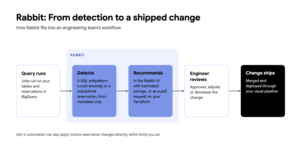
Rabbit implements this Tier 4 layer. It connects through Google Cloud APIs, with nothing to install for the base platform, and reads metadata (including the SQL text of your jobs) rather than your table rows or query results. Recommendations are the default: SQL antipatterns, partitioning and clustering, materialized views, and logical vs. physical storage billing. Automation is opt-in: Max Slot Optimizer for reservation max slots, the Job-level Pricing Model Optimizer to route each job to on-demand or a reservation, Reservation Optimizer for the reservation lifecycle, and Recommendation Applier, which opens pull requests that apply recommendations in your Terraform. Cost anomaly detection compares actual spend against a forecast and flags spikes. Because these levers interact, Rabbit optimizes across them rather than tuning one in isolation.
To see what your own bill could look like, try the BigQuery Savings Calculator.
How much can you save by optimizing BigQuery? Measure your progress with SQL
There is no universal number: savings depend on where you start and which tiers you have already worked through. On average, Rabbit users achieve a 32% reduction on their BigQuery costs. Measured savings include 47% at Nordstrom and 52% at Lufthansa Group with automation.
Averages only go so far, though. The number that matters is your own before and after. The three queries below give you that baseline: bytes billed over time, slot usage, and your most expensive queries. Run them before you start on Tier 1, then again after each change, and you’ll see which changes actually moved the bill.
Tracking bytes billed over time
Run this against the region-specific INFORMATION_SCHEMA view for the region where your jobs run (our example uses region-us). This view only covers the current project and the last 180 days, which is the INFORMATION_SCHEMA.JOBS retention limit, so don’t assume broader coverage. Bytes billed is the on-demand cost signal: for jobs running on a reservation you aren’t billed for bytes, so watch slot usage instead (next section). The query is project-level; to break it down by user, add user_email to the SELECT and GROUP BY.
SELECT DATE(creation_time) AS job_date, SUM(total_bytes_billed) / POW(2, 40) AS tib_billed, COUNT(*) AS job_countFROM `region-us`.INFORMATION_SCHEMA.JOBSWHERE creation_time BETWEEN TIMESTAMP_SUB(CURRENT_TIMESTAMP(), INTERVAL 30 DAY) AND CURRENT_TIMESTAMP() AND job_type = 'QUERY' AND statement_type != 'SCRIPT'GROUP BY job_dateORDER BY job_date DESCMonitoring slot utilization
These queries use total_slot_ms, which is available per job in INFORMATION_SCHEMA.JOBS. They help you tell whether you are overprovisioned (utilization well below your baseline) or underprovisioned (frequent queuing, or flat-lined at the ceiling).
The daily query shows the overall trend:
SELECT DATE(creation_time) AS job_date, SUM(total_slot_ms) / (1000 * 60 * 60 * 24) AS avg_slots_usedFROM `region-us`.INFORMATION_SCHEMA.JOBSWHERE creation_time BETWEEN TIMESTAMP_SUB(CURRENT_TIMESTAMP(), INTERVAL 30 DAY) AND CURRENT_TIMESTAMP() AND job_type = 'QUERY' AND statement_type != 'SCRIPT' AND DATE(creation_time) < CURRENT_DATE()GROUP BY job_dateORDER BY job_date DESCThe hourly query uses the same filters, truncated to the hour instead of the day, and excludes the current in-progress hour the same way the daily query excludes the current in-progress day. It is what surfaces the floor and ceiling signals from Tier 3: slot usage sitting flat at the max, and your lowest hourly usage over the last 2 to 4 weeks:
SELECT TIMESTAMP_TRUNC(creation_time, HOUR) AS job_hour, SUM(total_slot_ms) / (1000 * 60 * 60) AS avg_slots_usedFROM `region-us`.INFORMATION_SCHEMA.JOBSWHERE creation_time BETWEEN TIMESTAMP_SUB(CURRENT_TIMESTAMP(), INTERVAL 30 DAY) AND CURRENT_TIMESTAMP() AND job_type = 'QUERY' AND statement_type != 'SCRIPT' AND TIMESTAMP_TRUNC(creation_time, HOUR) < TIMESTAMP_TRUNC(CURRENT_TIMESTAMP(), HOUR)GROUP BY job_hourORDER BY job_hour DESCCompare this daily average, and your busiest hour, against your baseline. If the average sits well below the baseline most days, you are paying for slots you don’t use. Keep in mind that this is slot time your jobs consumed, not what you pay for: baseline slots bill whether or not queries use them. That gap is what you are looking for. To turn slot usage into a dollar figure per job, see what a BigQuery job actually costs on a reservation.
Identifying the costliest queries
This is the most actionable query in the section, because it tells you exactly where to look first. It lists the 20 most expensive completed queries from the last 7 days. The query field may be truncated for very long queries:
SELECT job_id, user_email, query, total_bytes_billed / POW(2, 30) AS gib_billed, creation_timeFROM `region-us`.INFORMATION_SCHEMA.JOBSWHERE creation_time > TIMESTAMP_SUB(CURRENT_TIMESTAMP(), INTERVAL 7 DAY) AND job_type = 'QUERY' AND state = 'DONE' AND statement_type != 'SCRIPT'ORDER BY total_bytes_billed DESCLIMIT 20If DDL and DML statements aren’t relevant to your cost review, you can add AND statement_type = 'SELECT' on top of the SCRIPT exclusion (not instead of it).
Summary: BigQuery cost optimization
Optimizing BigQuery is iterative. The teams making the most progress are the ones who know which queries to fix next. If you want to see where your bill is going before you start, the BigQuery Savings Calculator gives you an estimate based on your actual usage. To start realizing those savings, book a demo with the Rabbit team or start a free trial.