This post covers a specific optimization that’s available to teams on BigQuery capacity pricing with a slot commitment: routing individual queries to on-demand pricing to reduce autoscaling costs, without giving up the savings of your committed capacity.

Buying a slot commitment is often framed as the end of the BigQuery cost optimization story. You’ve locked in your capacity, you know what you’re paying, and you move on. But for most organizations, the bill doesn’t stop at the commitment — it keeps growing through autoscaling charges on top of it. This autoscaler waste is often the biggest remaining lever on BigQuery capacity pricing costs.

Most teams enable autoscaling to handle peak workloads, which is reasonable. But those charges can be significant if your workloads aren’t evenly distributed throughout the day.

Query-level pricing with committed slots: a different problem

BigQuery allows you to override the default reservation assignment on a per-query basis. This means a query that would normally run against your committed-slot reservation can instead be routed to on-demand pricing. There’s a full explanation of how this works in our post on dynamic job-level pricing optimization. If you’re not familiar with the mechanism, start there.

Learn more:
Unlock 15-20% Savings on BigQuery:
The Power of Dynamic, Job-Level Pricing Optimization

The short version: since queries have very different slot usage profiles, some queries process huge amounts of data with relatively simple transformations and are expensive on-demand but barely consume slots. Others read very little data but are slot-hungry. Routing the right queries to the right pricing model can reduce costs.

The catch with BigQuery slot commitments is that the optimization logic changes. When you’re on pure on-demand or autoscale-only pricing, the decision is straightforward: compare what the query costs on each model, pick the cheaper one. When you have committed slots, the math is different, and it doesn’t favor moving queries off reservation by default.

Here’s why: if a query runs during a period when your committed slots are underutilized, it costs you essentially nothing extra to run it on the reservation. You’ve already paid for those slots. Moving that query to on-demand means you pay twice: once for the commitment sitting idle, and again for the on-demand charge.

The only time it genuinely makes sense to move a query to on-demand is when that query is running during a period when your baseline is already fully utilized, and autoscaling is picking up the slack. In that case, the query is the marginal driver of the autoscaling cost, and moving it off the reservation eliminates that extra spend.

What does a query actually cost when you have a commitment?

Before identifying which queries to move, it helps to define what “cost” means in this context.

One useful frame is the effective slot-hour rate: the total cost of your setup (committed capacity plus autoscaling charges) divided by the actual slot-hours consumed by your workloads.

effective_slot_hour_rate =
  (SUM(cost of commitments) + SUM(cost of autoscaling))
  / SUM(total_slot_ms / 1000 / 60 / 60)

You can apply this rate to individual queries to get their slot-based cost: total_slot_ms / 1000 / 60 / 60 * effective_slot_hour_rate. This is the number that often surprises teams: a query that looks cheap on on-demand pricing can be consuming an enormous share of slot capacity.

Learn more about effective slot-hour cost:
What Does a BigQuery Job Actually Cost on a Reservation?

But this effective rate isn’t the right number for this particular optimization. What matters here is the marginal cost: the additional autoscaling spend caused by each query. That depends not just on the query itself, but on everything else running at the same time. A query running solo against a half-utilized baseline costs nothing extra. The same query running at peak load, when the baseline is already saturated, is directly causing the autoscaler to provision more slots.

How well is your BigQuery commitment actually utilized?

To find the queries worth moving, you first need to understand how your committed capacity is being used over time. Specifically, which hours have idle baseline slots versus which hours are burning autoscaling budget.

This query joins RESERVATIONS_TIMELINE and JOBS_TIMELINE_BY_ORGANIZATION from INFORMATION_SCHEMA to give you an hourly breakdown of how your slots were actually used. It assumes your baselines assigned across reservations sum to your committed capacity (a best practice), and that idle slot sharing is enabled.

Replace ADMIN_PROJECT, EDITION, and REGION with your own values before running. (BigQuery will likely show a very large byte estimate for this query, but usually the actual billed amount will be much smaller – in our case, it was 3% of the estimate).

WITH res_minute AS (
  SELECT
    rt.period_start AS minute_start,
    rt.reservation_id,
    rt.edition,
    rt.slots_assigned AS baseline_slots,
    COALESCE(SAFE_DIVIDE(rt.period_autoscale_slot_seconds, 60.0), 0) AS autoscale_slots,
    COALESCE(rt.max_slots, rt.slots_assigned + COALESCE(rt.autoscale.max_slots, 0)) AS max_slots,
  FROM `ADMIN_PROJECT.region-REGION`.INFORMATION_SCHEMA.RESERVATIONS_TIMELINE rt
  WHERE rt.period_start >= TIMESTAMP_SUB(CURRENT_TIMESTAMP(), INTERVAL 30 DAY)
  AND rt.edition='EDITION'

),

job_minute AS (
  SELECT
    TIMESTAMP_TRUNC(jt.period_start, MINUTE) AS minute_start,
    jt.reservation_id,
    SUM(jt.period_slot_ms) / 60000.0 AS used_slots,
  FROM `region-REGION`.INFORMATION_SCHEMA.JOBS_TIMELINE_BY_ORGANIZATION jt
  WHERE jt.period_start >= TIMESTAMP_SUB(CURRENT_TIMESTAMP(), INTERVAL 30 DAY)
    AND jt.job_creation_time >= TIMESTAMP_SUB(CURRENT_TIMESTAMP(), INTERVAL 32 DAY)
    AND (jt.statement_type IS NULL OR jt.statement_type != 'SCRIPT')
  GROUP BY 1, 2
),

agg_minute AS (
  SELECT
    r.minute_start,
    r.edition,
    SUM(r.baseline_slots) AS total_committed,
    SUM(r.autoscale_slots) AS total_autoscale,
    SUM(r.max_slots) AS max_slots,
    COALESCE(SUM(j.used_slots), 0) AS total_used,
  FROM res_minute r
  LEFT JOIN job_minute j USING (minute_start, reservation_id)
  GROUP BY r.minute_start, r.edition
),

slot_split AS (
  SELECT
    minute_start,
    edition,
    LEAST(total_used, total_committed) AS used_committed_slots,
    GREATEST(total_committed - total_used, 0) AS wasted_committed_slots,
    GREATEST(total_used - total_committed, 0) AS used_autoscale_slots,
    total_autoscale - GREATEST(total_used - total_committed, 0) AS wasted_autoscale_slots,
    max_slots,
  FROM agg_minute
)

SELECT
  TIMESTAMP_TRUNC(minute_start, HOUR) AS period_start,
  edition,
  ROUND(AVG(used_committed_slots), 1) AS used_committed_slots,
  ROUND(AVG(wasted_committed_slots), 1) AS wasted_committed_slots,
  ROUND(AVG(used_autoscale_slots), 1) AS used_autoscale_slots,
  ROUND(AVG(wasted_autoscale_slots), 1) AS wasted_autoscale_slots,
  ROUND(AVG(max_slots), 1) AS max_slots,
FROM slot_split
GROUP BY 1, 2
ORDER BY period_start;

Filter the results to a single edition and render the output as a stacked bar chart. You should see something like the image below, where each bar represents an hour and the colored segments break down how your slots were actually used:

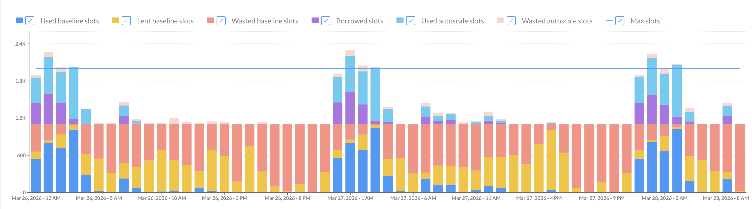
Reading the chart:

• Red bars (wasted committed slots) are your sunk cost: you paid for that capacity and didn’t use it. During these hours, running additional queries on reservation costs you nothing extra. This is not where you’re looking for on-demand candidates.
• Light blue and light orange peaks show hours where autoscaling kicked in. These are the hours you should focus on: queries running here are the ones driving extra cost beyond your commitment.
• Bars with both red and autoscale segments are interesting edge cases. The hourly average can obscure short bursts: a single hour might have 40 minutes of idle baseline followed by 20 minutes of heavy autoscaling. If you strip out the hourly grouping from the query above and drop to per-minute data, you can see these intra-hour patterns clearly.

If you see the same usage shape repeating week over week, that’s a signal: your autoscaling peaks are driven by predictable, recurring workloads — exactly the kind of queries that are worth targeting.

Which queries are worth moving from a BigQuery commitment to on-demand?

Good candidates for on-demand routing share a few characteristics: they run on a predictable schedule (typically orchestrated by Airflow or dbt), they process similar volumes on each run, and their on-demand cost is meaningfully lower than the autoscaling cost they’re causing.

The last point is crucial. The comparison isn’t between on-demand cost and the query’s full slot-based cost — it’s between on-demand cost and the marginal autoscaling cost: how much additional autoscaling this specific query triggers, given everything else running at the same time. A query that uses 500 slot-hours might cause only 50 of those to land in autoscale territory, depending on the hour it runs. That’s the number you need.

The query below computes this marginal cost per query group (grouped by normalized query hash, project, and user), and compares it against the on-demand equivalent. (Depending on your setup, a different grouping may be more useful: for example, if you have labels that identify each step of your pipelines, such a step may be a natural way to group.) Results are ranked by estimated savings if moved. A positive est_savings_if_moved means moving the query to on-demand would, historically, have saved money.

Replace ADMIN_PROJECT, REGION, and the payg_rate (cost of a slot-hour on your edition type) and on_demand_cost_per_tb params with your actual rates before running. The PAYG autoscale rate and on-demand rate vary by edition and region — check the current GCP pricing page for your values.

WITH params AS (
  SELECT
    0.06 AS payg_rate,
    6.25 AS on_demand_cost_per_tb,
),

res_minute AS (
  SELECT
    rt.period_start AS minute_start,
    rt.reservation_id,
    rt.slots_assigned AS baseline_slots,
    COALESCE(SAFE_DIVIDE(rt.period_autoscale_slot_seconds, 60.0), 0) AS autoscale_slots,
  FROM `ADMIN_PROJECT.region-REGION`.INFORMATION_SCHEMA.RESERVATIONS_TIMELINE rt
  WHERE rt.period_start >= TIMESTAMP_SUB(CURRENT_TIMESTAMP(), INTERVAL 30 DAY)
),

all_jobs_minute AS (
  SELECT
    TIMESTAMP_TRUNC(jt.period_start, MINUTE) AS minute_start,
    jt.reservation_id,
    SUM(jt.period_slot_ms) / 60000.0 AS used_slots,
  FROM `region-REGION`.INFORMATION_SCHEMA.JOBS_TIMELINE_BY_ORGANIZATION jt
  WHERE jt.period_start >= TIMESTAMP_SUB(CURRENT_TIMESTAMP(), INTERVAL 30 DAY)
    AND jt.job_creation_time >= TIMESTAMP_SUB(CURRENT_TIMESTAMP(), INTERVAL 32 DAY)
    AND jt.parent_job_id IS NULL
  GROUP BY 1, 2
),

capacity_minute AS (
  SELECT
    r.minute_start,
    SUM(r.baseline_slots) AS total_committed,
    SUM(r.autoscale_slots) AS total_autoscale,
    COALESCE(SUM(j.used_slots), 0) AS total_used,
  FROM res_minute r
  LEFT JOIN all_jobs_minute j USING (minute_start, reservation_id)
  GROUP BY r.minute_start
),

raw_jobs AS (
  SELECT
    j.job_id,
    j.project_id,
    j.user_email,
    j.reservation_id,
    j.creation_time,
    j.query_info.query_hashes.normalized_literals AS query_norm_hash,
    j.labels,
    COALESCE(j.total_bytes_billed, 0) / 1e12 * p.on_demand_cost_per_tb AS on_demand_cost,
  FROM `region-REGION`.INFORMATION_SCHEMA.JOBS_BY_ORGANIZATION j
  CROSS JOIN params p
  WHERE j.creation_time >= TIMESTAMP_SUB(CURRENT_TIMESTAMP(), INTERVAL 30 DAY)
    AND j.job_type = 'QUERY'
    AND j.state = 'DONE'
    AND j.cache_hit IS NOT TRUE
    AND j.error_result IS NULL
    AND j.reservation_id IS NOT NULL
    AND j.parent_job_id IS NULL
    AND j.query_info.query_hashes.normalized_literals IS NOT NULL
),

query_groups AS (
  SELECT
    query_norm_hash,
    project_id,
    user_email,
    ARRAY_AGG(DISTINCT job_id) AS job_ids,
    max_by(labels, creation_time) AS labels, -- takes the labels from the latest run, use it to identify your query
    COALESCE(SUM(on_demand_cost), 0) AS query_on_demand_cost,
    COUNT(*) AS runs,
    MAX_BY(reservation_id, creation_time) AS reservation_id,
  FROM raw_jobs
  GROUP BY 1, 2, 3
  HAVING COUNT(*) >= 2
),

query_minute AS (
  SELECT
    qg.query_norm_hash,
    qg.project_id,
    qg.user_email,
    TIMESTAMP_TRUNC(jt.period_start, MINUTE) AS minute_start,
    SUM(jt.period_slot_ms) / 60000.0 AS query_used_slots,
  FROM query_groups qg
  CROSS JOIN UNNEST(qg.job_ids) AS jid
  INNER JOIN `region-REGION`.INFORMATION_SCHEMA.JOBS_TIMELINE_BY_ORGANIZATION jt
    ON jt.job_id = jid
  WHERE jt.job_creation_time >= TIMESTAMP_SUB(CURRENT_TIMESTAMP(), INTERVAL 32 DAY)
    AND jt.period_start >= TIMESTAMP_SUB(CURRENT_TIMESTAMP(), INTERVAL 30 DAY)
    AND jt.parent_job_id IS NULL
  GROUP BY 1, 2, 3, 4
),

marginal AS (
  SELECT
    qm.query_norm_hash,
    qm.project_id,
    qm.user_email,
    SUM(
      LEAST(qm.query_used_slots, GREATEST(cm.total_used - cm.total_committed, 0))
    ) / 60.0 * p.payg_rate AS marginal_cost,
  FROM query_minute qm
  INNER JOIN capacity_minute cm USING (minute_start)
  CROSS JOIN params p
  GROUP BY 1, 2, 3, p.payg_rate
)

SELECT
  qg.query_norm_hash AS deparametrized_query_hash,
  qg.project_id,
  qg.user_email,
  qg.runs,
  qg.reservation_id,
  labels,
  ARRAY(SELECT * FROM UNNEST(job_ids) LIMIT 5) AS job_ids,
  ROUND(qg.query_on_demand_cost, 2) AS on_demand_cost,
  ROUND(m.marginal_cost, 2) AS marginal_cost,
  ROUND(m.marginal_cost - qg.query_on_demand_cost, 2) AS est_savings_if_moved,
FROM query_groups qg
INNER JOIN marginal m USING (query_norm_hash, project_id, user_email)
WHERE m.marginal_cost > qg.query_on_demand_cost
ORDER BY est_savings_if_moved DESC;

The queries at the top of the list are your primary candidates. You can identify them using the labels or the job_ids. The JOBS_BY_ORGANIZATION view doesn’t let us view the query string itself, but you can run a follow-up query in the specific project_id.region-REGION.INFORMATION_SCHEMA.JOBS view to get the query string as well.

One important caveat on the granularity of this analysis: while BigQuery’s slot usage data is available at the second level, there’s too much variance between individual runs of the same query to base decisions on second-by-second data. A minute-level approximation is more stable and sufficient for this purpose. Properly configured max-slots settings also flatten the sharpest peaks, which reduces the sensitivity to sub-minute timing anyway.

The savings ceiling you need to understand

Looking at the query results, it’s tempting to take the whole list and flip everything to on-demand in one pass. Don’t.

Here’s why: the marginal cost of each query is calculated against historical data where all other queries were still running on reservation. Once you move a query off reservation, the total slot pressure changes, which changes the marginal cost calculation for every remaining query.

A simple example: imagine two queries running simultaneously, each consuming 500 slots, while your committed baseline is 400. Together, they’re pulling 600 slots from autoscaling. Moving one to on-demand eliminates its 500 slots from the reservation, freeing the remaining query’s autoscaling exposure to drop significantly — but not to zero, because the other query is still there. Moving both at the same time doesn’t save 500 + 500 = 1,000 autoscale slots. It saves at most 600, the actual autoscale usage (remember, your baseline is 400). And if the savings from moving both are less than the combined on-demand costs, you might not save anything at all.

There’s also a hard boundary: baseline slots are always paid for, even when idle. Your on-demand savings can never exceed your total autoscaling spend. Once autoscaling is eliminated, the optimization ceiling is reached.

This means there’s no single query that returns the globally optimal set of queries to move. It’s an iterative problem by nature.

How to move BigQuery queries from a reservation to on-demand?

The practical approach:

1. Pick the top query from the savings query output above. This is a greedy heuristic: it doesn’t find the global optimum, but it’s a good approximation and a safe starting point.

2. Route it to on-demand. You can do this by adding SET @@reservation = 'none'; at the start of the query, or by setting the reservation field in the JobConfiguration to ‘none’ when submitting the job via the API. If you’re using Airflow or dbt, this means modifying the job configuration before execution.

3. If you’re handling multiple candidates, you can switch a handful at the same time, provided they run at different hours and don’t overlap at peak periods. If they share the same window, treat them sequentially.

4. Wait and observe. Give it at least a week (or longer for monthly pipelines). Your usage patterns need time to normalize before you rerun the analysis.

5. Rerun the savings query against the new period to identify the next set of candidates. Repeat until the incremental savings become small enough that the effort isn’t worth it.

This is deliberately conservative. The goal is to make real, measurable reductions in autoscaling spend, not to optimize on paper and hope the math holds in production.

How Rabbit handles this automatically

Doing this manually is genuinely difficult. The marginal cost calculation is inherently approximate, the interactions between queries make it non-linear, and the iterative loop (switch, wait, measure, repeat) requires sustained attention across multiple weeks.

Rabbit approaches this differently. Rather than relying on a static snapshot of historical data, Rabbit analyzes your reservations, commitments, and query patterns globally and runs a simulation that models how queries interact with each other. This allows it to identify a set of candidates that can be moved together (not just the top query in isolation) without overcounting the expected savings.

Instead of moving one query and waiting a week to see the effect, Rabbit can show you the projected savings per user and per project across a batch of candidates, and let you configure the scope: which projects and users to include in the optimization.

On the execution side, you don’t need to manually update job configurations in your orchestrator. Rabbit’s open-source Airflow plugin and dbt adapter integrate directly into your pipelines and set the optimal pricing model at runtime dynamically, based on the current utilization of your committed capacity at the moment the job runs. If your commitment has idle slots available right now, the query stays on reservation. If the baseline is saturated, the query routes to on-demand. Setup takes about five minutes and requires no manual job-level overrides going forward.

Rabbit also tracks the realized savings over time, so you can validate results against actual billing data rather than relying purely on the pre-move estimate.

This optimization works best when approached as an ongoing process, not a one-time project. Workloads change, pipelines get added, and what was optimal three months ago may not be optimal today. The manual approach is tedious and error-prone, which is why we’re automating this optimization with Rabbit.

Ready to try Rabbit? Sign up for free or book a demo to walk through your specific setup with our team.