This post covers how to decide whether a BigQuery commitment is worth it, and how to size one without locking in avoidable waste for the next 1-3 years. Read on for a practical workflow: how to measure slot usage second by second, simulate candidate commitment sizes, and pressure-test the result before you buy.

Commitments are often treated like a simple discount decision: “we are on reservations, so let’s commit and save.” In practice, this is where many teams create a new fixed cost line they cannot unwind. They buy a pool based on averages, then keep paying autoscaling on peak windows anyway. The result is the worst of both worlds: idle committed slots plus expensive pay-as-you-go autoscale on top.

Learn more:
How to Cut BigQuery Autoscaling Costs When You Have a Commitment

What are you actually buying with a BigQuery commitment?

On BigQuery Enterprise and Enterprise Plus, capacity commitments are a way to save on BigQuery capacity-based compute once you are already using reservations. They let you lock a slot quantity for 1 or 3 years at a discounted rate compared with pay-as-you-go capacity pricing (exact discounts depend on term, edition, and region — check the pricing page for your setup). The discount is real – but so is the lock-in.

A few details to consider:

• Commitments are tied to an admin project, edition, and region.
• You can reassign committed capacity across reservations, but you cannot “return” purchased slots during the term (1 or 3 years).
• Committed slots are billed continuously, whether or not they are used in that second.
• If demand exceeds committed baseline and autoscaling is enabled, overage is still billed separately at pay-as-you-go capacity rates (i.e. without the commitment discounts).

That last point is where teams get surprised: a commitment does not magically cap your bill. If peaks still drive autoscaling, you can end up paying for committed capacity and pay-as-you-go autoscale on top. The costliest pattern we see is sizing off overall averages without checking how often demand actually sits above the commitment level you are considering.

So the question is not “Do I get a discount with commitments?”. The real question is: Will this commitment stay utilized enough, often enough, to beat paying for bursty demand on autoscale?

When does a BigQuery commitment help and when does it hurt?

The key driver is the shape of your workloads, not total slot-hours. Two workloads can consume the same monthly slot-hours and still produce opposite commitment outcomes:

• A flatter workload can keep committed slots busy and capture most of the discount.
• A bursty workload can leave committed slots idle for long periods, then spill to autoscale on peaks.

Let’s consider the following scenario comparing bursty vs flat usage, outlined in one of our previous posts:

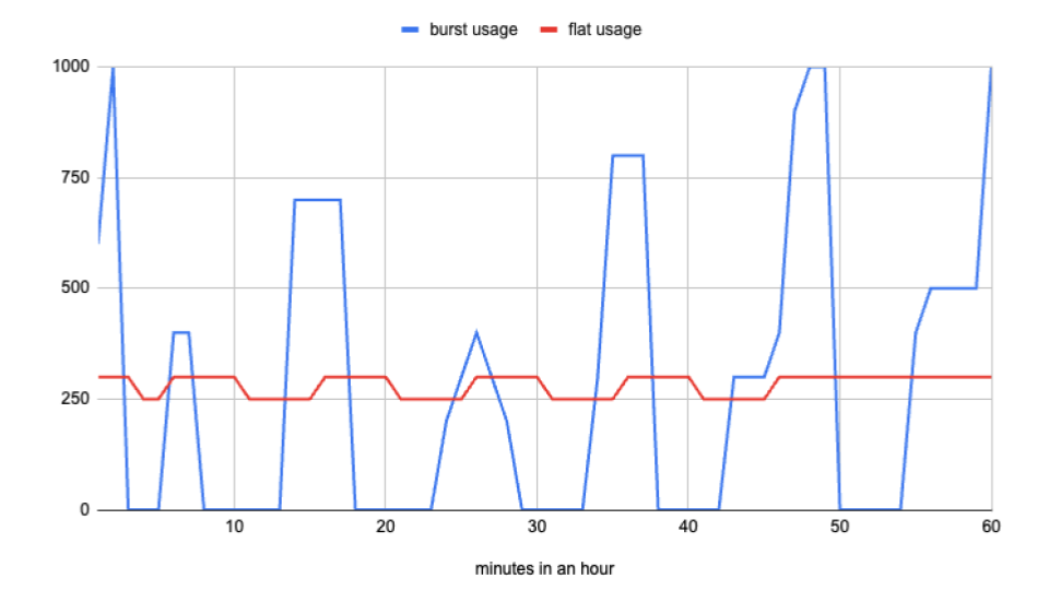
• Two patterns with the same total slot-hours in a month can have roughly the same cost with no commitment (about $12.1K in this stylized example).
• In the bursty pattern, even a 50-slot commitment can make costs worse: total cost rises by about 6% to around $12.8K.
• In the flat pattern, committing to 250 slots on a 1-year term can reduce cost by around 18% to about $10K.

Real usage is messier than any single chart. That is why a single monthly aggregate is not enough. You need to know, second by second, how often your demand sits above or below each commitment level you are considering.

Learn more:
BigQuery Capacity-based Pricing: How to Optimize Your Reservation Cost

How to right-size a BigQuery commitment?

Let’s walk through the same sequence we use when helping teams avoid overcommitment:

1. Build a second-by-second demand series for the commitment pool you are sizing.
2. Run a sweep of candidate commitment sizes and compare estimated totals (including autoscale overage).
3. Calibrate the autoscale waste assumption using reservation timeline data (no guesswork).
4. Read the outputs: look for the inflection point where extra commitment buys mostly idle capacity.
5. Reduce waste levers before you lock in for a 1- or 3-year term (max slots, scheduling, dynamic pricing).
6. Roll out commitments in stages and re-check the simulation against reality.

The sections below guide you through that process.

Step 1: Analyze your usage (per-second demand)

Before deciding on any commitment size, build a per-second view of how much slot capacity your workloads actually consume. Step 2 runs a SQL sweep that simulates cost at each commitment level you sweep (the per-second aggregation is the seconds_usage CTE inside that same query).

• Source data: INFORMATION_SCHEMA.JOBS_TIMELINE_BY_ORGANIZATION, aggregated as SUM(period_slot_ms) for each second.
• Scope rule: commitments are global to one admin project + edition + region pool, not one reservation. Run one simulation per real pool.
• If you have multiple editions or separate commitment pools, do not sum everything together. Filter with reservation_id, project, or labels so each run maps to one real pool.
• Include committed_slots = 0 in your sweep. This is your no-commitment baseline and keeps the comparison honest.

Step 2: Simulate candidate commitment sizes

Once you have per-second demand, simulate a grid of commitment sizes and compare estimated totals.

Query setup:

• Replace [REGION] so it matches where the commitment lives.
• Edit params: window, pay-as-you-go and annual or three-year committed slot-hour rates, autoscale_waste_ratio.
• By default we keep reservation_id IS NOT NULL — so you only see jobs already on a reservation. On-demand jobs disappear from the picture unless you comment that out or add filters for specific reservations, projects, etc., depending on what you are trying to size.
• GENERATE_ARRAY(0, …, 50) — start at 0 (no commitment), then 50, 100, … (in the query below, the upper bound is currently 500 — raise/lower it if your peaks require a wider sweep).
• Permissions: Jobs timeline by organization

Output: one row per candidate commitment size (committed_slots), with commitment_cost, autoscale_cost, commitment_utilization_percent, and estimated_total, ordered from smallest to largest commitment.

-- Simulates total capacity cost ≈ (committed pool × commitment rate × hours)
--   + (per-second autoscaled slice × pay-as-you-go rate), with the autoscaled part padded with an 18% waste
-- Single statement: edit `params` and `[REGION]`. Optionally restrict or relax `reservation_id` filter (see WHERE).
-- Slot-hour rates: https://cloud.google.com/bigquery/pricing#capacity_compute_pricing

WITH params AS (
  SELECT
    TIMESTAMP_SUB(CURRENT_TIMESTAMP(), INTERVAL 7 DAY) AS analysis_start,
    CURRENT_TIMESTAMP() AS analysis_end,
    0.06 AS pay_as_you_go_slot_hour_rate,
    0.048 AS commit_slot_hour_rate, -- 20% discount with 1-year, 40% with 3-year commit, compared to pay-as-you-go
    0.18 AS autoscale_waste_ratio  -- Optimal setup: 18%, typical setup: 30%, but extremely bursty usage can be more than 90%
),
seconds_usage AS (
  SELECT
    period_start,
    SUM(period_slot_ms) / 1000.0 AS used_slots
  FROM `region-[REGION]`.INFORMATION_SCHEMA.JOBS_TIMELINE_BY_ORGANIZATION j
  CROSS JOIN params p
  WHERE period_start >= p.analysis_start
    AND period_start < p.analysis_end
    AND job_creation_time >= TIMESTAMP_SUB(p.analysis_start, INTERVAL 6 HOUR)
    AND job_type = 'QUERY'
    AND (statement_type != 'SCRIPT' OR statement_type IS NULL)
    -- To include ALL jobs (on-demand and reservation), comment out the line below:
    AND reservation_id IS NOT NULL
    -- To limit to specific reservations, add a filter such as:
    -- AND reservation_id IN ('admin_project:[REGION].res_a', 'admin_project:[REGION].res_b')
  GROUP BY period_start
),
window_bounds AS (
  SELECT
    TIMESTAMP_DIFF(p.analysis_end, p.analysis_start, SECOND) / 3600.0 AS window_hours
  FROM params p
),
commitment_candidates AS (
  SELECT slot_count
  FROM UNNEST(GENERATE_ARRAY(0, 500, 50)) AS slot_count
),
cost_by_candidates AS (
  SELECT
    c.slot_count AS committed_slots,
    w.window_hours * c.slot_count * p.commit_slot_hour_rate AS commitment_cost,
    COALESCE(
      SUM(
        GREATEST(COALESCE(u.used_slots, 0) - c.slot_count, 0) / (1.0 - p.autoscale_waste_ratio)
      ) / 3600.0 * p.pay_as_you_go_slot_hour_rate,
      0
    ) AS autoscale_cost,
    IF(
      c.slot_count = 0,
      CAST(NULL AS FLOAT64),
      100.0 * COALESCE(SUM(LEAST(COALESCE(u.used_slots, 0), c.slot_count)), 0)
        / (CAST(c.slot_count AS FLOAT64) * w.window_hours * 3600.0)
    ) AS commitment_utilization_percent
  FROM commitment_candidates c
  CROSS JOIN window_bounds w
  CROSS JOIN params p
  LEFT JOIN seconds_usage u ON TRUE
  GROUP BY
    c.slot_count,
    w.window_hours,
    p.commit_slot_hour_rate,
    p.pay_as_you_go_slot_hour_rate,
    p.autoscale_waste_ratio
)
SELECT
  committed_slots,
  commitment_cost,
  autoscale_cost,
  commitment_utilization_percent,
  commitment_cost + autoscale_cost AS estimated_total
FROM cost_by_candidates
ORDER BY committed_slots;

The model above is rough but practical:

1. The pool is always on: commitment_cost = committed slots x window hours x discounted commitment slot-hour rate.
2. Anything above the commitment in a given second is modeled as pay-as-you-go: autoscale_cost = usage above commitment (max(used - committed, 0)) priced at pay-as-you-go rates.
3. Add a default autoscale waste value to only the autoscaled slice (default 0.18, or used / 0.82 equivalent). For a more accurate value, see Step 3 about measuring your autoscaler waste.
4. commitment_utilization_percent: of the committed slot-seconds you are paying for in the window, what share did jobs actually use (capped at the commitment per second)? NULL when commitment is zero. Seconds missing from the timeline count as zero usage.
5. Compare estimated_total = commitment_cost + autoscale_cost across candidates.

This is a planning model, not an invoice replica. Sanity-check rates with Google’s pricing or calibrate rates with your actual billing setup, and validate your assumptions with your finance team.

Step 3: Measure your actual autoscale waste

The commitment query assumes 18% autoscale waste, which is useful as a starting point – while that’s not measured in the sizing query in Step 2, it is what we’ve observed across many optimal setups. Your real autoscale waste can be much higher if max_slots is loose or workload spikes are sharp.

Measure your own baseline with a quick join between RESERVATIONS_TIMELINE and JOBS_TIMELINE_BY_ORGANIZATION, then feed that ratio back into the sizing model:

Output: one row per reservation_id with billed vs consumed autoscale slot-seconds and an autoscale_waste_ratio you can plug into autoscale_waste_ratio in Step 2.

-- Per-reservation autoscale waste over the last 7 days.
-- Edit [REGION]. Optionally narrow to specific reservation_ids.
-- Permissions: bigquery.reservations.list + jobs timeline org-level read.

WITH params AS (
  SELECT
    TIMESTAMP_SUB(CURRENT_TIMESTAMP(), INTERVAL 7 DAY) AS analysis_start,
    CURRENT_TIMESTAMP() AS analysis_end
),
billed_autoscale AS (
  SELECT
    reservation_id,
    period_start,
    slot_capacity AS baseline_slots,
    period_autoscale_slot_seconds AS billed_autoscale_slot_seconds
  FROM `region-[REGION]`.INFORMATION_SCHEMA.RESERVATIONS_TIMELINE
  CROSS JOIN params p
  WHERE period_start >= p.analysis_start
    AND period_start < p.analysis_end
),
job_usage AS (
  SELECT
    j.reservation_id,
    j.period_start,
    SUM(j.period_slot_ms) / 1000.0 AS used_slots
  FROM `region-[REGION]`.INFORMATION_SCHEMA.JOBS_TIMELINE_BY_ORGANIZATION j
  CROSS JOIN params p
  WHERE j.period_start >= p.analysis_start
    AND j.period_start < p.analysis_end
    AND j.job_creation_time >= TIMESTAMP_SUB(p.analysis_start, INTERVAL 6 HOUR)
    AND j.job_type = 'QUERY'
    AND (j.statement_type != 'SCRIPT' OR j.statement_type IS NULL)
  GROUP BY j.reservation_id, j.period_start
),
consumed_autoscale AS (
  SELECT
    j.reservation_id,
    TIMESTAMP_TRUNC(j.period_start, MINUTE) AS minute_start,
    SUM(GREATEST(j.used_slots - b.baseline_slots, 0)) AS consumed_autoscale_slot_seconds
  FROM job_usage j
  INNER JOIN billed_autoscale b
    ON j.reservation_id = b.reservation_id
    AND TIMESTAMP_TRUNC(j.period_start, MINUTE) = b.period_start
  GROUP BY j.reservation_id, minute_start
)
SELECT
  b.reservation_id,
  SUM(b.billed_autoscale_slot_seconds) AS billed_autoscale_slot_seconds,
  COALESCE(SUM(c.consumed_autoscale_slot_seconds), 0) AS consumed_autoscale_slot_seconds,
  SAFE_DIVIDE(
    SUM(b.billed_autoscale_slot_seconds)
      - COALESCE(SUM(c.consumed_autoscale_slot_seconds), 0),
    SUM(b.billed_autoscale_slot_seconds)
  ) AS autoscale_waste_ratio
FROM billed_autoscale b
LEFT JOIN consumed_autoscale c
  ON b.reservation_id = c.reservation_id
  AND b.period_start = c.minute_start
GROUP BY b.reservation_id
HAVING SUM(b.billed_autoscale_slot_seconds) > 0
ORDER BY autoscale_waste_ratio DESC;

How to interpret the waste query output:

• autoscale_waste_ratio = fraction of billed autoscale slot-seconds that jobs did not consume. 0.18 means 18% waste — matches our default assumption. If yours says 0.30, plug 0.30 into the commitment query’s autoscale_waste_ratio parameter instead of 0.18.
• Lower is better — it means BigQuery’s autoscaler closely tracked real demand. High waste usually points to a max slots config that is too generous or bursty workloads with long ramp-down tails.
• If a reservation shows very high waste (>40%), that is a strong signal to tune max slots before you commit: you would be paying commitment prices on top of an already-leaky autoscaler.

If your measured ratio is closer to 0.30 than 0.18, re-run the commitment model with 0.30. One parameter change can materially alter the best commitment size.

Step 4: Read the results without overcommitting

Treat each row as a what-if scenario, then inspect three columns together:

• estimated_total: the directional winner for this historical window.
• commitment_utilization_percent: how much of the committed capacity you paid for was actually used (see Step 2 for the exact definition).
• autoscale_cost: how much burst spend remains after commitment.

How to interpret the sweep output:

• Each row is a what-if commitment size. committed_slots = 0 is the no-commitment baseline: you are not buying a pool, and autoscale_cost is the whole story.
• Compare commitment_cost vs autoscale_cost: are you mainly buying a pool, or paying for spikes?
• If commitment_utilization_percent is low on a large commitment, you bought a lot of idle capacity.
• Lowest estimated_total wins, assuming your usage patterns in the next term look like the window you analyzed.

Common patterns to be aware of:

• Spiky usage: the best row is often committed_slots = 0. If you only need a big pool briefly, prepaying for a large flat commitment can lose to pay-as-you-go autoscale (even with the waste bump), because you end up buying idle committed slot-seconds you rarely use.
• Increasing commitment from zero to a moderate level often drops autoscale_cost sharply.
• High commitment setting: past a point, autoscale_cost flattens but commitment_cost keeps rising linearly.
• Utilization falls as you increase commitment, and savings disappear.

That inflection point is where many teams overbuy.

Step 5: Before you sign, optimize first

Commitment sizing should come after you reduce obvious waste drivers. Three high-impact levers:

1. Tune reservation max_slots so autoscaling does not over-provision by default. A loose max is one of the fastest ways to push real autoscale waste far above the default 18% assumption, which means the 0.82 gross-up mental model is wrong for your environment. Use the Step 3 query to measure your actual autoscale waste per reservation, then plug that measured ratio back into Step 2.
2. Shift predictable batch workloads out of shared peak windows when possible. The goal is to flatten the curve: move slot demand out of shared peaks so more seconds sit under a smaller commitment. In practice, that scheduling work is often what flips the answer from “commitment does not pay” to “now it does” — without buying a bigger flat pool than you actually need.
3. Apply dynamic job-level pricing so each query can run on the cheaper model for its context, especially when autoscale is doing real work on top of a commitment.

Learn more:
Unlock 15-20% Savings on BigQuery: The Power of Dynamic, Job-Level Pricing Optimization

How to roll out BigQuery commitments in practice?

Avoid all-in commitment changes unless your workload is highly stable and your confidence is high.

A staged rollout is a safe approach:

• Start with a smaller commitment.
• Observe at least one full usage cycle (weekly and monthly jobs included).
• Compare realized spend versus simulation.
• Increase in controlled increments only if the utilization pattern holds.

If you decide a commitment makes sense, a good practice is to stagger it over time: instead of creating one huge commitment up front, create a smaller one first. Watch how it shows up on the bill, validate the effect against your Step 2 sweep, and re-run the analysis: do the recommended numbers still look right in production, or did reality move?

From there, keep going gradually. One practical pattern teams use is to split the total into multiple smaller purchases on a cadence (for example, instead of one large yearly commit on day one, layering six smaller commitments every ~2 months so you can repeatedly re-check reality against the simulation as you approach your steady-state target). The goal is to preserve optionality: you still honor the full term for each purchased commitment, but you avoid locking the largest possible number before you have high confidence the utilization pattern will hold.

Past manual analysis: how Rabbit helps

Manually, this process is doable but time-consuming: extract timeline data, calibrate waste assumptions, run scenarios, validate after rollout, then repeat as workloads change.

Rabbit helps across that full loop:

• Reservations insights show slot usage and autoscaler waste so you can see where commitment value is leaking.
• Commitments recommendations help identify where 1- or 3-year commitments make sense based on historical behavior.
• Reservation Planner recommends better baseline and max slot settings to reduce waste before commitment decisions.
• Dynamic job-level pricing automation routes queries between on-demand and capacity-based pricing based on what is cheaper in context.

The practical effect: you can treat commitment planning as an ongoing optimization process, not a one-time spreadsheet exercise – fully automatically, without having to sacrifice engineering hours on continuous optimization.